This assignment involved analysing and exploring Hawaii's climate data in 2 steps:
- Climate Analysis and Exploration
- Climate App
Python and SQLAlchemy was used to do basic climate analysis and data exploration of the given climate database. All of the analysis was completed using SQLAlchemy ORM queries, Pandas, and Matplotlib.
- The datetime library was used to identify the date 12 months prior to the last date available. Using these dates and after dropping null values, the precipitation values for the last year of data was used to plot the following graph:
- A statistics summary using .describe() revealed the following:


This section asked to find the number of stations (nine) and the most active station (USC00519281).
Temperature observations at this station for the last 12 months was plotted as a histogram with the following results:

This is a web app in the app.py file, created using SQLAlchemy and Flask API. The climate database can be queried for the following to receive information in JSON format:
- Precipitation (/api/v1.0/precipitation): This route displays every date and temperature observation across all weather stations in Hawaii.
- Stations (/api/v1.0/stations): This route displays a list of all 9 stations (ID, Station and Name).
- Temperature Observations (/api/v1.0/tobs): This route displays every date and temperature observation for the most active station in Hawaii (USC00519281) in the last 12 months of data available.
- Daily Normals from start date (/api/v1.0/start_date): This route allows you to enter a start date in the format 'YYYY-MM-DD' to retrieve daily normals (TMIN, TAVG, TMAX) from that date onward until the end of data available.
- Daily Normals between start and end date (/api/v1.0/start_date/end_date): This route allows you to enter a start date AND an end date in the format 'YYYY-MM-DD' to retrieve daily normals (TMIN, TAVG, TMAX) for the date range.
June and December temperature observations were retrieved by converting string dates to DateTime objects to filter queries by month.
The average temperature in June at all stations across all available years in the dataset is 74.94 (F). And the average temperature in June at all stations across all available years in the dataset is 71.04 (F). Thus, the mean temperature difference between June and December is a mere 3.9 degrees Fahrenheit.
In this analysis, the t-test was paired because the samples do not have any data overlap. The high t-value shows the two sets are very different, while the low p-value shows that the data did not occur by chance.

This challenge involved using a predefined function that calculated daily normals for a given date range (2018-06-01 to 2018-06-15). The .timedelta() method from the datetime library was also used to determine matching start and end dates from the previous year.
With the daily normals, the following graph was plotted using tavg, tmin and tmax values:

In this challenge, the first task was to calculate the precipitation for each weather station and display the results and station information. After querying the databases for both tables and checking for null values, the query results were saved in Pandas data frames to make it easier to manipulate data using groupby and merge. The next data frame is the result:

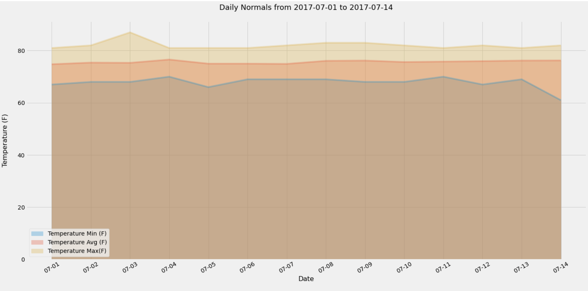
The second part of this challenge involved finding daily normals for each date of our defined trip from 2017-07-01 to 2017-07-14 (using only the month and day to identify historic data with the same dates) and plotting an area plot as below:
Trip daily normals dataframe:
